RF
RFIIR Filter Design in Python: LPF, HPF, BPF, BSF
Advertisement
This article provides Python code for simulating IIR (Infinite Impulse Response) filters, covering Low-Pass Filter (LPF), High-Pass Filter (HPF), Band-Pass Filter (BPF), and Band-Stop Filter (BSF) types. You’ll find the code, explanations, and the resulting plots generated by the script.
Introduction to IIR Filters
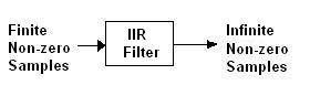
Unlike FIR (Finite Impulse Response) filters, IIR filters use current input sample values, past input samples, and past output samples to calculate the current output sample value. This feedback mechanism is what gives IIR filters their “infinite” impulse response.
Here’s a visual representation of an IIR filter:

A simple IIR equation can be represented as follows:
Where:
- is the current output sample.
- is the current input sample.
- are the feedforward coefficients.
- are the feedback coefficients.
For more information on the differences between FIR and IIR filters, refer to resources comparing the two.
IIR Filter Python Code
Below is the Python code that implements the LPF, HPF, BPF, and BSF filters. It leverages the scipy.signal library for filter design and matplotlib for plotting the frequency responses.
import matplotlib.pyplot as plt
import scipy.signal as sig
import numpy as np
from math import pi

plt.close('all')

# IIR filter design as per Butterworth specifications
Fs = 1000  # Sampling frequency
n = 7  # Number of orders of the filter
fc = 100  # Cutoff frequency of the filter (For LPF/HPF)
fc1 = np.array([200, 400])  # Start and Stop frequencies for BPF/BSF
w_c = 2 * fc/Fs
w_c1 = 2 * fc1/Fs

# IIR filter configurations of different types
[b1, a1] = sig.butter(n, w_c, btype='lowpass')
[b2, a2] = sig.butter(n, w_c, btype='highpass')
[b3, a3] = sig.butter(n, w_c1, btype='bandpass')
[b4, a4] = sig.butter(n, w_c1, btype='bandstop')

# Frequency response of IIR filter (LPF type)
[w1, h1] = sig.freqz(b1, a1, worN=2000)
w_lpf = Fs*w1/(2*pi)
h_db_lpf = 20 * np.log10(abs(h1))

# Frequency response of IIR filter (HPF type)
[w2, h2] = sig.freqz(b2, a2, worN=2000)
w_hpf = Fs*w2/(2*pi)
h_db_hpf = 20 * np.log10(abs(h2))

# Frequency response of IIR filter (BPF type)
[w3, h3] = sig.freqz(b3, a3, worN=2000)
w_bpf = Fs*w3/(2*pi)
h_db_bpf = 20 * np.log10(abs(h3))

# Frequency response of IIR filter (BSF type)
[w4, h4] = sig.freqz(b4, a4, worN=2000)
w_bsf = Fs*w4/(2*pi)
h_db_bsf = 20 * np.log10(abs(h4))

# Plots
figure, axis = plt.subplots(2, 2)

axis[0, 0].plot(w_lpf, h_db_lpf)
axis[0, 0].set_title("IIR filter response (LPF type)")
axis[0, 0].set_xlabel("Frequency (Hz)")
axis[0, 0].set_ylabel("Magnitude (dB)")

axis[0, 1].plot(w_hpf, h_db_hpf)
axis[0, 1].set_title("IIR filter response (HPF type)")
axis[0, 1].set_xlabel("Frequency (Hz)")
axis[0, 1].set_ylabel("Magnitude (dB)")

axis[1, 0].plot(w_bpf, h_db_bpf)
axis[1, 0].set_title("IIR filter response (BPF type)")
axis[1, 0].set_xlabel("Frequency (Hz)")
axis[1, 0].set_ylabel("Magnitude (dB)")

axis[1, 1].plot(w_bsf, h_db_bsf)
axis[1, 1].set_title("IIR filter response (BSF type)")
axis[1, 1].set_xlabel("Frequency (Hz)")
axis[1, 1].set_ylabel("Magnitude (dB)")

plt.tight_layout()
plt.show()
IIR Filter Python Output Plots
The code generates four plots, one for each filter type, showing the frequency response (Magnitude in dB vs. Frequency in Hz). The x-axis represents frequency in Hertz (Hz), and the y-axis represents the magnitude in decibels (dB).
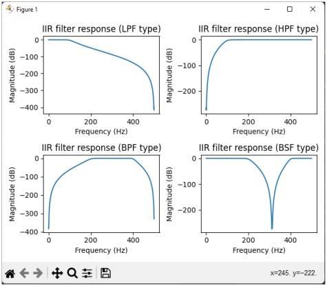
These plots visually demonstrate how each filter attenuates or passes different frequency components of a signal.
Advertisement