RF
RFLow Pass FIR Filter Implementation in MATLAB
Advertisement
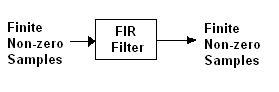
This section covers MATLAB source code for implementing a Low Pass FIR Filter. It discusses filter design using the firrcos function and the MATLAB FDA tool.
Using the FIRRCOS MATLAB Function
clc;
clear all;
close all;
FFT_size = 1024;
t = 0:0.001:(FFT_size - 1) / 1000;
x = sin(2 * pi * 50 * t) + sin(2 * pi * 200 * t);
coeff = firrcos(50, 100, 50, 1000);
y = conv(x, coeff);
y1 = fft(y, 1024);
figure;
plot(abs(fft(x, 1024)));
figure;
plot(abs(y1));
Here, the input signal x consists of two sinusoidal waves at 50 Hz and 200 Hz. The goal is to pass this signal through a low-pass FIR filter, eliminating frequencies above the cutoff frequency. The length of the FFT is 1024.
This implementation uses the MATLAB pre-defined function firrcos to generate the filter coefficients:
coeff = firrcos(n, fc, bw, fs);
Where:
n: The order of the filter (a positive integer).fc: The cutoff frequency of the filter (must be greater than 0 and less than fs/2).bw: The transition bandwidth (must be greater than 0, and[fc-bw/2, fc+bw/2]must fall within the range[0, fs/2]).fs: The sampling frequency (must be greater than 0).
We also use the conv pre-defined function to convolve the input signal with the coefficients to get the time-domain output:
y = conv(x, coeff);
Where:
x: The input signal.coeff: The filter coefficients.
After obtaining the convolution output (y), the code plots the FFT output alongside the FFT of the input signal. The FFT is used to convert the time-domain signal into the frequency domain.

Figure 1: Input signal (x) in the frequency domain at 50 Hz and 200 Hz. The right-side peaks are the mirror image of the original input signal.
Below is the output signal (y) in the frequency domain. From these two figures, we can see that the peak at 200 Hz is eliminated because it’s above the cutoff frequency (100 Hz).

Figure 2: Output signal (y) in the frequency domain.
Note: If an input signal of 110 Hz is used, and the cutoff frequency is 100 Hz, the input signal will not be completely eliminated in the output. This is because it takes time to decay completely, a period known as the transition period.
Implementing a Low Pass FIR Filter in MATLAB using the FDA Tool
clear all;
close all;
clc;
FFT_size = 1024;
t = 0:0.001:(FFT_size - 1) / 1000;
x1 = sin(2 * pi * 15 * t) + sin(2 * pi * 100 * t);
x1 = x1 / 2;
%%fs = 1000 Hz, fpass = 50 Hz, fstop = 100 Hz
b = [
    -0.00075204 -0.0034964  -0.0025769  -0.0029542  -0.0019023  7.5785e-005
    0.0029216 0.0060432   0.0086036   0.0096315   0.0082863   0.0041324
    -0.0026099  -0.010933   -0.019081   -0.024793   -0.025704   -0.019846
    -0.0061564  0.015154    0.042456    0.072834    0.1025  0.12742 0.14402
    0.14984 0.14402 0.12742 0.1025  0.072834    0.042456    0.015154
    -0.0061564  -0.019846   -0.025704   -0.024793   -0.019081   -0.010933
    -0.0026099  0.0041324   0.0082863   0.0096315   0.0086036   0.0060432
    0.0029216   7.5785e-005 -0.0019023  -0.0029542  -0.0025769  -0.0034964
    -0.00075204
];
b_dec = b * (32768);
b_deca = b_dec(:);
x_dec = x1 * (32768);
x_decaa = x_dec(:);
x = [
    0 0 0 0 0 0 0 0 0 0 0 0 0 0 0 0 0 0 0 0 0 0 0 0 0 0 0 0 0 0 0 0 0 0 0 0 0 0 0 0 0 0 0 0 0 0 0 0 0 0
    0   0   0   x1
];
for k = 55:1077
    y(k) = (x(k) * b(1))    + ...
           (x(k - 1) * b(2))  + ...
           (x(k - 2) * b(3))  + ...
           (x(k - 3) * b(4))  + ...
           (x(k - 4) * b(5))  + ...
           (x(k - 5) * b(6))  + ...
           (x(k - 6) * b(7))  + ...
           (x(k - 7) * b(8))  + ...
           (x(k - 8) * b(9))  + ...
           (x(k - 9) * b(10))  + ...
           (x(k - 10) * b(11))  + ...
           (x(k - 11) * b(12))  + ...
           (x(k - 12) * b(13))  + ...
           (x(k - 13) * b(14))  + ...
           (x(k - 14) * b(15))  + ...
           (x(k - 15) * b(16))  + ...
           (x(k - 16) * b(17))  + ...
           (x(k - 17) * b(18))  + ...
           (x(k - 18) * b(19))  + ...
           (x(k - 19) * b(20))  + ...
           (x(k - 20) * b(21))  + ...
           (x(k - 21) * b(22))  + ...
           (x(k - 22) * b(23))  + ...
           (x(k - 23) * b(24))  + ...
           (x(k - 24) * b(25))  + ...
           (x(k - 25) * b(26))  + ...
           (x(k - 26) * b(27))  + ...
           (x(k - 27) * b(28))  + ...
           (x(k - 28) * b(29))  + ...
           (x(k - 29) * b(30))  + ...
           (x(k - 30) * b(31))  + ...
           (x(k - 31) * b(32))  + ...
           (x(k - 32) * b(33))  + ...
           (x(k - 33) * b(34))  + ...
           (x(k - 34) * b(35))  + ...
           (x(k - 35) * b(36))  + ...
           (x(k - 36) * b(37))  + ...
           (x(k - 37) * b(38))  + ...
           (x(k - 38) * b(39))  + ...
           (x(k - 39) * b(40))  + ...
           (x(k - 40) * b(41))  + ...
           (x(k - 41) * b(42))  + ...
           (x(k - 42) * b(43))  + ...
           (x(k - 43) * b(44))  + ...
           (x(k - 44) * b(45))  + ...
           (x(k - 45) * b(46))  + ...
           (x(k - 46) * b(47))  + ...
           (x(k - 47) * b(48))  + ...
           (x(k - 48) * b(49))  + ...
           (x(k - 49) * b(50));
    y_dec = y * 32768;
    y_deca = y_dec(:);
end
z = y(51:end);
y1 = fft(z, 1024);
figure;
plot(abs(fft(x1, 1024)));
figure;
plot(abs(y1));
y1_dec = y1 * 32768;
y1_deca = y1_dec(:);
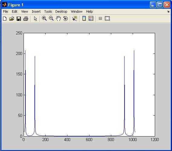
Figure 3: Input signal in the frequency domain at 15 Hz and 100 Hz.
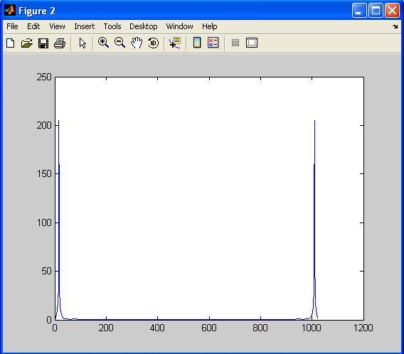
Figure 4: Output signal (y) in the frequency domain at 15 Hz.
From the above two figures, we can conclude that the input signal at 100 Hz frequency is getting cut off at the output. In this implementation, we are using the FDA (Filter Design Analysis) tool to generate the filter coefficients. The specifications of this filter are:
- Fs = 1000 Hz
- Fpass = 50 Hz
- Fstop = 100 Hz
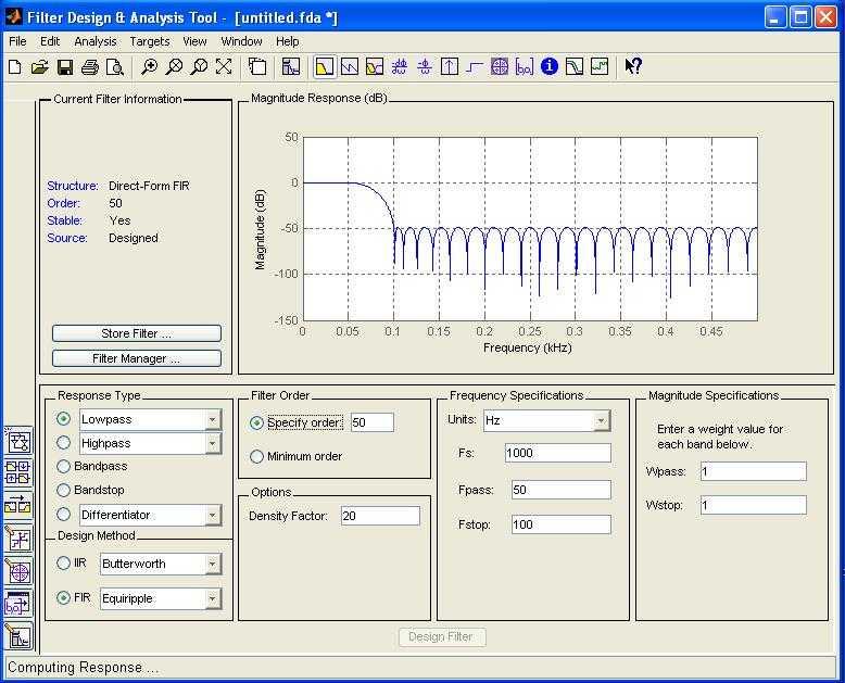
Figure 5: FDA tool to generate coefficients for low pass FIR filter.
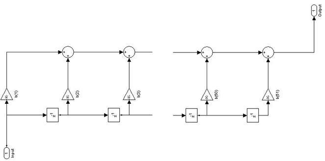
Figure 6: Structure of Low pass FIR filter.
In this implementation, the length of the FFT is 1024. The input signal x1 consists of two sine waves at 15 Hz and 100 Hz:
x1 = sin(2 * pi * 15 * t) + sin(2 * pi * 100 * t);
The input signal is scaled because if the input (x) is not in the Q-15 format range (i.e., -1 to 0.9999999), we divide x by 2 (i.e., x1/2). The coefficients are then assigned to ‘b’.
Zero-padding is performed for x1 because the filter equation multiplies previous input signals with coefficients.
The filter equation is designed for a Low pass FIR filter of order ‘50’. The ‘k’ value starts from 55 because the original input signal starts from the 55th location in MATLAB and ends at the 1077th location. The filter equation is implemented as follows:
If the first input comes, it’s multiplied with the first coefficient. The remaining coefficients are multiplied with previous inputs, which have a value of ‘0’. If the second input comes, it’s multiplied with the first coefficient, and the first input is multiplied with the second coefficient. The remaining coefficients are multiplied with previous inputs, which have a value of ‘0’. This process continues until all inputs are processed, and the coefficients are repeated periodically.
Finally, the code plots the FFT of the input and output values.
Advertisement