Analog Filter Design and Implementation in MATLAB

This document provides MATLAB code examples for designing and simulating analog low-pass and high-pass filters. Let’s dive into the implementations.

Analog Low Pass Filter MATLAB Code

clc;
close all;
clear all;
f=100:20:8000;
fh=900;
k=length(f);

for i=1:k
  m(i)=1/sqrt(1+(f(i)/fh)^2);
  mag(i)=20*log10(m(i));
end

figure;
semilogx(f,mag);
title('Magnitude Response of Analog Low Pass Filter')
xlabel('Frequency----->');
ylabel('Magnitude in dB');
grid on;

This code calculates and plots the magnitude response of an analog low-pass filter. Here’s a breakdown:

• clc; close all; clear all;: Clears the command window, closes all figures, and clears all variables from the workspace. This is standard practice to ensure a clean environment.
• f=100:20:8000;: Defines a frequency vector f ranging from 100 Hz to 8000 Hz with a step of 20 Hz. This is the range over which the frequency response will be plotted.
• fh=900;: Sets the cutoff frequency fh to 900 Hz. This is a key parameter determining the filter’s behavior.
• k=length(f);: Determines the length of the frequency vector f and stores it in k.
• The for loop calculates the magnitude response:
  • m(i)=1/sqrt(1+(f(i)/fh)^2);: This is the transfer function of a first-order low-pass filter. It calculates the magnitude m(i) at each frequency f(i).
  • mag(i)=20*log10(m(i));: Converts the magnitude m(i) to decibels (dB).
• The figure; semilogx(f,mag); commands create a new figure and plot the magnitude response in dB against frequency (on a logarithmic scale for the frequency axis).
• The remaining commands add a title, axis labels, and a grid to the plot for better readability.

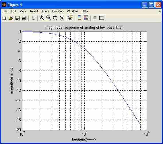
Here’s the expected output plot:

The plot shows the typical frequency response of a low-pass filter, where frequencies below the cutoff frequency are passed with little attenuation, while frequencies above the cutoff frequency are increasingly attenuated.

Analog High Pass Filter MATLAB Code

clc;
close all;
clear all;
f=100:20:8000;
fl=400;
k=length(f);

for i=1:k
  m(i)=1/sqrt(1+(fl/f(i))^2);
  mag(i)=20*log10(m(i));
end

figure;
semilogx(f,mag);
title('Magnitude Response of Analog High Pass Filter');
xlabel('Frequency----->');
ylabel('Magnitude in dB');
grid on;

This code is very similar to the low-pass filter code, but it implements a high-pass filter. Here’s a breakdown of the key differences:

• fl=400;: Sets the cutoff frequency fl to 400 Hz.
• m(i)=1/sqrt(1+(fl/f(i))^2);: This is the transfer function of a first-order high-pass filter. Notice that fl is now in the numerator of the fraction inside the square root, which is the crucial difference that makes it a high-pass filter.

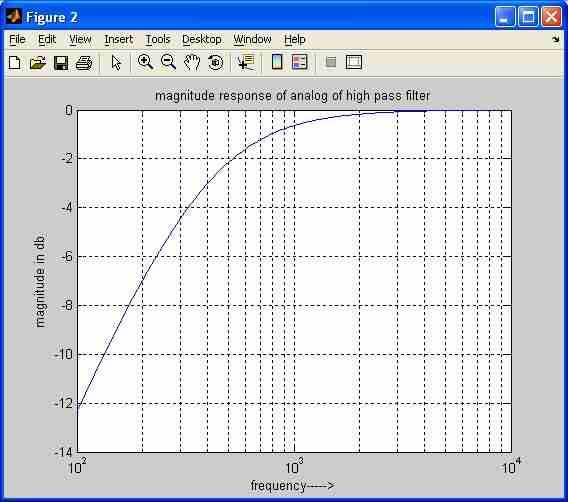
Here’s the expected output plot:

The plot shows the typical frequency response of a high-pass filter, where frequencies above the cutoff frequency are passed with little attenuation, while frequencies below the cutoff frequency are increasingly attenuated.