Convolution in Python: NumPy vs. Brute Force Implementation

This article explores implementing convolution in Python, comparing the efficiency and results of using NumPy’s np.convolve function with a more direct, “brute-force” method. Convolution is a fundamental operation, especially in fields like signal processing and image analysis. It’s used, for example, to simulate channel impairments on time-domain transmit sequences like those found in OFDM/OFDMA systems.

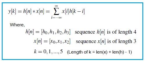
For Linear Time-Invariant (LTI) systems, convolution allows us to determine the output sequence ($y[n]$) given a channel impulse response ($h[n]$) and an input sequence ($x[n]$). The convolution is mathematically represented as follows.

Python Convolution Script

The Python script below demonstrates two ways to perform convolution: using NumPy’s optimized np.convolve and a brute-force implementation. You can easily switch between real and complex number inputs.

import numpy as np
import matplotlib.pyplot as plt

# Inputs as complex numbers
#x = np.random.normal(size=3) + 1j * np.random.normal(size=3)  # normal random complex vectors
#h = np.random.normal(size=4) + 1j * np.random.normal(size=4)  # normal random complex vectors

# Inputs as real numbers
x = [20,31,56]   # Time domain sequence say in OFDM Transmitter
h = [10,2,5,8]   # Time domain channel impulse response

L = len(x) + len(h) - 1  # length of convolution output

# Method-1 : Python convolution function from NumPy module
y3 = np.convolve(h, x)
print("y3=", y3)

# Method-2 : Convolution using Brute-force method
N = len(x)
M = len(h)
y = np.zeros(L)  # array filled with zeros
for i in np.arange(0,N):
    for j in np.arange(0,M):
        y[i + j] = y[i + j] + x[i] * h[j]
print("y=",y)

#Difference between NumPy module and Brute-force method
y2 = y-y3

# Initialise the subplot function using number of rows and columns
figure, axis = plt.subplots(2, 2)

# For Built in convolution
axis[0,0].plot(y3)
axis[0,0].set_title("Method # 1 : np.convolve")

# For Our own function
axis[0,1].plot(y)
axis[0,1].set_title("Method # 2 : Brute-force method")

#Difference between two
axis[1, 0].plot(y2)
axis[1, 0].set_title("Difference between both methods")

plt.show()

The script first defines two input vectors, x and h, representing the input sequence and channel impulse response, respectively. The length of the convolution output L is calculated.

Two methods are then used to compute the convolution:

• Method 1: np.convolve: This utilizes NumPy’s built-in convolve function, which is highly optimized for performance.
• Method 2: Brute-Force: This method directly implements the convolution formula using nested loops. For each element in x and h, the product is added to the appropriate index in the output array y.

Finally, the script calculates the difference between the results of the two methods (y2) and plots the outputs of both methods alongside their difference for comparison.

Inputs for Real Numbers

The following vectors are used as inputs for the convolution of real numbers.

x = [20,31,56]   #Time domain sequence say in OFDM Transmitter
h = [10,2,5,8]   #Time domain channel impulse response

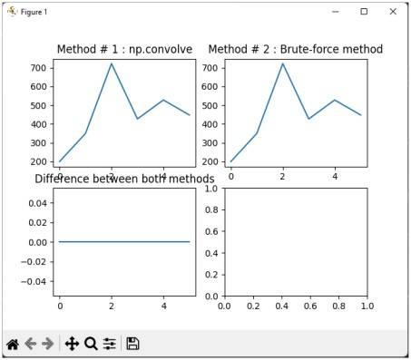
Output for Convolution of Real Numbers

The plot below shows the output of the convolution when both inputs x and h contain real numbers.

Inputs for Complex Random Numbers

To experiment with complex numbers, uncomment the following lines in the script:

x = np.random.normal(size=3) + 1j * np.random.normal(size=3)  # normal random complex vectors
h = np.random.normal(size=4) + 1j * np.random.normal(size=4)  # normal random complex vectors

These lines generate random complex vectors for x and h.

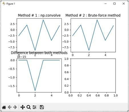
Output for Convolution of Complex Numbers

The resulting plot displays the convolution output when the inputs x and h are complex numbers.

Conclusion

This example provides a practical comparison between NumPy’s np.convolve and a brute-force convolution implementation for both real and complex numbers. NumPy’s function is highly optimized for speed and efficiency, making it the preferred choice for most applications. The brute-force method, while less efficient, helps illustrate the underlying principles of convolution.