Butterworth Filter Design in MATLAB: Low-Pass and High-Pass

This article presents MATLAB code for designing Butterworth Low-Pass and High-Pass filters.

Butterworth Low-Pass Filter MATLAB Code

%Butterworth Low Pass Filter
clc;
close all;
clear all;
format long;
rp=input('enter the passband ripple:(default:0.15)');
rs=input('enter the stopband ripple:(default:60)');
wp=input('enter the passband frequency:(default:1500)');
ws=input('enter the stopband frequency:(default:3000)');
fs=input('enter the sampling frequency:(default:7000)');
w1=2*wp/fs;
w2=2*ws/fs;
[n,wn]=buttord(w1,w2,rp,rs,'s');
[z,p,k]= butter(n,wn);
[b,a]=butter(n,wn,'s');
w=0:0.01:pi;
[h,om]=freqs(b,a,w);
m=20*log10(abs(h));
an=angle(h);
subplot(2,1,1);
plot(om/pi,m);
ylabel('gain in db--------->');
xlabel('(a) normalized freq------>');
subplot(2,1,2);
plot(om/pi,an);
ylabel('phase in db--------->');
xlabel('(b) normalized freq------>');

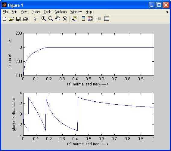
The code above implements a Butterworth Low-Pass filter. It takes passband ripple (rp), stopband ripple (rs), passband frequency (wp), stopband frequency (ws), and sampling frequency (fs) as inputs. The buttord function determines the filter order (n) and cutoff frequency (wn). The butter function then calculates the filter coefficients (b and a). Finally, the frequency response is computed and plotted.

Here’s an example of the output plot:

Butterworth High-Pass Filter MATLAB Code

%Butterworth High Pass Filter
clc;
close all;
clear all;
format long;
rp=input('enter the passband ripple:(default:0.2)');
rs=input('enter the stopband ripple:(default:40)');
wp=input('enter the passband frequency:(default:2000)');
ws=input('enter the stopband frequency:(default:3500)');
fs=input('enter the sampling frequency:(default:8000)');
w1=2*wp/fs;
w2=2*ws/fs;
[n,wn]=buttord(w1,w2,rp,rs,'s');
[z,p,k]= butter(n,wn);
[b,a]=butter(n,wn,'high','s');
w=0:0.01:pi;
[h,om]=freqs(b,a,w);
m=20*log10(abs(h));
an=angle(h);
subplot(2,1,1);
plot(om/pi,m);
ylabel('gain in db--------->');
xlabel('(a) normalized freq------>');
subplot(2,1,2);
plot(om/pi,an);
ylabel('phase in db--------->');
xlabel('(b) normalized freq------>');

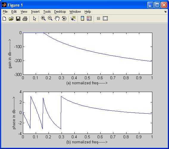
The code above implements a Butterworth High-Pass filter. The structure is similar to the low-pass filter, but the butter function is called with the 'high' argument to specify a high-pass filter design.

Here’s an example of the output plot: