MATLAB Code for Simulating Phase Noise Impairment
Advertisement
This section details MATLAB source code demonstrating local oscillator phase noise impairment and its effect on the constellation diagram. The MATLAB code is broken into parts, with Part A and Part C being identical to those mentioned on the AWGN page (not included here).
Part B: Main Script
Phase_noise_dBc = -25; % integrated phase noise in dBc
Phase_noise_cutoff = 1000e2; % cutoff frequency of PSD
Phase_noise_floor = -125; % phase noise floor in dBc/Hz
Phase_noise_fs = 100e6; % sampling frequency

in=mapper_out_ori; %Assuming mapper_out_ori is defined earlier
in=in';
out=RX_PN(in,Phase_noise_dBc,Phase_noise_cutoff,Phase_noise_floor,Phase_noise_fs);

figure;
plot(real(out),imag(out),'c+');
title('constellation with phase noise');


## RX_PN.m: Function to Add Phase Noise

```matlab
function out = RX_PN(in,dBc, cutoff, floor, Fs)
[M N] = size(in);
ltx = 2^(fix(log2(M-0.5))+2); % ltx will always be at least 2xM
if cutoff/(Fs/ltx)<16,
    ltx = 16*Fs/cutoff;
    ltx = 2^(fix(log2(ltx-0.5))+1);
end

PhaseNoise = frequency_synth_lorenzian(dBc, cutoff, floor, Fs, ltx).';
Nphn = length(PhaseNoise);

if Nphn<M
    error(['Phase noise vector must be longer than' num2str(Nsamples)])
end

Nstart = fix(rand(1,1)*(Nphn-M)); % random staring point
PhaseNoise = PhaseNoise(Nstart:Nstart+M-1);

% Add phase noise to data
out = zeros(size(in));
for k=1:N
    out(:,k) = in(:,k).*PhaseNoise.';
end
frequency_synth_lorenzian.m: Function to Generate Lorentzian Phase Noise
function y = frequency_synth_lorenzian( K, B, p2, Fs, ltx);
global d
Ns = ltx; % Number of samples for ifft calculation
df = Fs/Ns; % frequency resolution
k = [0:1:Ns/2-1, -Ns/2:1:-1]; % frequency index range
% frequency range: f = k * df

p2o = p2;
p2 = 10^(p2/10); % in V^2/Hz
p2 = p2*df; % in V^2/df

Ko = K;
K = 10^(K/10); % in V^2
B = B/df; % 3-dB bandwidth index

% Low frequency part is defined by Lorenzian function
SSBmask = sqrt( K*B/pi./([1:Ns/2].^2+B^2) );

% High frequency part is defined by the noise floor of the system p2
SSBmask = max(SSBmask, sqrt(p2)*ones(size(SSBmask)));

%-- Phase noise PHI(f, f>0) is first generated as a wide band signal
PHI = sqrt(0.5) * abs( randn(1,Ns/2) + j*randn(1,Ns/2) );
PHI = PHI .* exp(j*2*pi*rand(1,Ns/2));

%-- Phase noise PHI(f, f>0) is shaped according to the wanted mask
PHI = PHI .* SSBmask;

%-- Phase noise PHI(f) is then generated from PHI(f, f>0)
% (no phase noise on the carrier)
PHI = [0 PHI(1:Ns/2-1) conj(PHI(Ns/2:-1:1))];

NoisePower = 10*log10( sum(abs(PHI).^2) );

if (0)
    f = k(2:Ns/2)*df;
    PHI_f = 20*log10(abs(PHI(2:Ns/2))/sqrt(df));
    SSBmask_f = 20*log10(SSBmask(1:Ns/2-1)/sqrt(df));
    % normalisation to get PHI(f) in dBc/Hz, and not dBc/df
    figure(20),semilogx(f, PHI_f, 'b-','linewidth',1);
    hold on; grid on; zoom on;
    semilogx(f, SSBmask_f, 'r-','linewidth', 2);
    axis([f(1) f(end) p2o-10 SSBmask_f(1)+10]);
end;

%-- Correction for the integrated phase noise power:
PHI = PHI * 10^((Ko-NoisePower)/20);

%-- Phase noise phi(t) in the time domain
phi = ifft(PHI,Ns)*Ns;

%-- Local oscillator signal lo(t) in the time domain
lo = exp(j*phi);

%-- Local oscillator signal LO(f) in the frequency domain
if (0)
    LO = fft(lo,Ns)/Ns;
    f = k(2:Ns/2)*df;
    LO_f = 20*log10(abs(LO(2:Ns/2))/sqrt(df));
    SSBmask_f = 20*log10(SSBmask(1:Ns/2-1)/sqrt(df));
    figure(21);semilogx(f, LO_f, 'k-','linewidth',1);
    hold on; grid on; zoom on;
    semilogx(f, SSBmask_f, 'r-','linewidth',2);
    axis([f(1) f(end) p2o-10 SSBmask_f(1)+10]);
end;

%-- Prepare lo(t) for efficient use in dbbm_fe
y = lo(1,1:ltx*fix(Ns/ltx));
y = reshape(y,ltx,fix(Ns/ltx));
Explanation
This code simulates the impact of phase noise on a communication system’s constellation diagram. It does this by:
-
Generating Phase Noise: The
frequency_synth_lorenzianfunction creates a phase noise signal with a Lorentzian power spectral density (PSD). The PSD is defined by the integrated phase noise (K), cutoff frequency (B), and noise floor (p2). The function synthesizes the phase noise in the frequency domain and then transforms it to the time domain using an inverse FFT. -
Applying Phase Noise: The
RX_PNfunction applies the generated phase noise to the input signal (in). It randomly selects a starting point within the phase noise vector and multiplies the input signal by the complex exponential of the phase noise. -
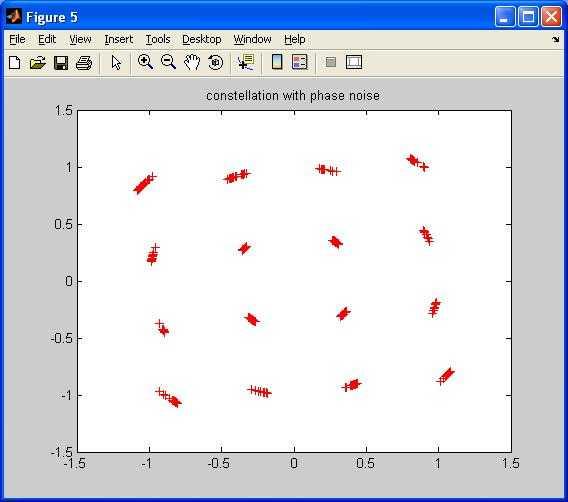
Visualizing the Constellation: The main script plots the real and imaginary components of the output signal (
out), creating a constellation diagram that visually represents the effect of phase noise.
Input and Output Constellation Diagrams
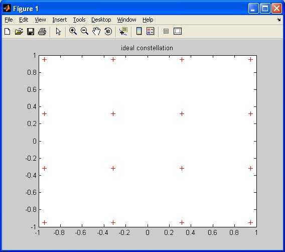
Input Constellation Diagram:

Output Constellation Diagram (with Phase Noise):

As you can see from the output constellation diagram, the phase noise causes the constellation points to spread out, degrading the signal quality.
Reference
The code is adapted from the book “Digital Front-End Compensation for Emerging Wireless Systems” by François Horlin and André Bourdoux.
Advertisement
 RF
RF


