 RF
RFUnderstanding RF Filters: Design, Types, and Applications
Advertisement
An RF (Radio Frequency) filter is an electronic component used in wireless communication systems to pass a desired range of frequencies while blocking undesired frequencies.
RF filters play a crucial role in radio transmitters and receivers to ensure efficient signal transmission and reception, respectively. There are several types of RF filters, such as Low Pass Filters, High Pass Filters, Band Pass Filters, and Band Stop Filters, each with distinct characteristics.
RF filter design requires a deep understanding of RF concepts, circuit design, and practical implementation considerations based on the desired filter type and specifications.
The diagram below shows an RF up-converter, which converts an IF (Intermediate Frequency) signal to an RF signal using a heterodyne approach with two RF mixers. This example is the transmitter part of a C-band RF transceiver used in VSAT (Very Small Aperture Terminal) systems. The IF input frequency range is from 52 to 88 MHz, and the RF output frequency range is from 5925 to 6425 MHz.
In this RF up-converter design, there are three RF filters: a low pass filter (LPF) at the input, a band pass filter (BPF) after the first mixer, and another BPF after the second mixer. At the input, a 52-88 MHz low pass filter is used, built with discrete components. This signal is mixed with a 1112.5 MHz signal, resulting in a 1182.5 MHz signal output along with other mixer products. After the first mixer, a BPF (band pass filter) that passes 1182.5 MHz with a bandwidth of 36MHz is used. Later, after the second mixing stage, a 5925 to 6425 MHz microstrip-based parallel-coupled band pass filter is incorporated.
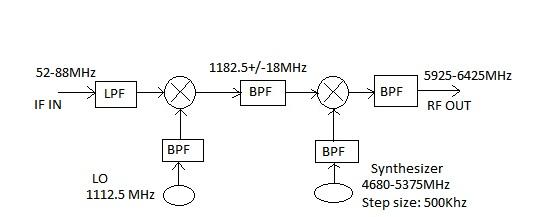
In the first stage of mixing, a local oscillator with a fixed value of 1112.5MHz is passed through a microstrip-based 3-4 stage hairpin RF filter. A round corner edge-coupled band pass filter of microstrip type is used to filter the synthesizer output, which ranges from 4680 to 5375MHz.
RF Low Pass Filter Design Example
Let’s consider an example of RF low pass filter design with the following specifications:
- Impedance: 50 Ohm
- Cutoff frequency (Fc): 3 GHz
- Equi-ripple: 0.5dB
- Rejection: 40 dB at 2*Fc
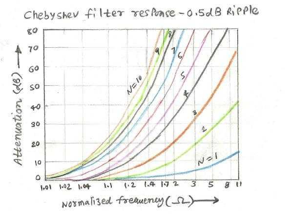
Step 1: Determine the normalized frequency, which in this case is w/wc, equal to 2 (6GHz/3GHz). Then, determine the filter type based on the required ripple. In this case, with approximately 0.5dB of ripple, a Chebyshev topology filter is ideal.
There are various filter topologies, such as Butterworth, Chebyshev, Bessel, or Elliptic. The appropriate topology is chosen based on the filter type and design specifications.
Now, based on the normalized frequency (2) and attenuation (40dB), and using the filter response curve (Chebyshev LPF with 0.5 dB ripple), determine the filter order (N) required for the design. The filter response will have normalized frequency on the X-axis and Attenuation on the Y-axis. Different filter orders are plotted against these two. Using 40dB and a normalized frequency of 2, we obtain a filter order of 5 from the curve for our RF filter design.
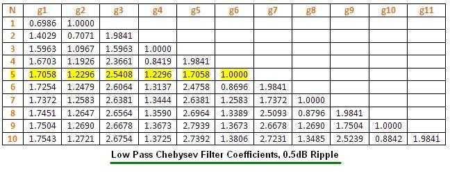
Based on the filter order N (here 5) and using the Filter coefficients table as mentioned above for Chebyshev LPF for 0.5dB ripple, we determine the filter coefficients, which are g1=1.7058, g2=1.2296, g3=2.5408, g4=1.2296, g5=1.7058, g6=1.
The figure above mentions Low Pass Chebyshev Filter Coefficients for 0.5dB ripple for various orders of the filter. The following figure mentions an LPF with order N using discrete L and C components.
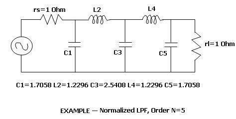
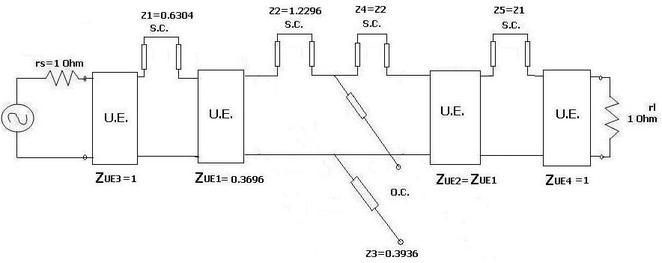
Step 2: Now use Richard’s transformation to replace an inductor with a short circuit line and a capacitor with an open circuit line. The length of the lines should be λ/8. The figure below is obtained after Richard’s transformation is applied to the discrete circuit for RF filter design.
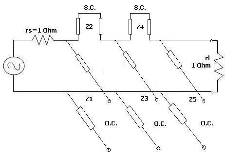
Step 3: Now convert all the short-circuited stubs, which are in series, into shunt-connected open circuit stubs. This can be achieved using Kuroda’s identities. This is depicted in the figures below. To apply Kuroda’s identity, unit elements are introduced in the circuit wherever required, as shown in the figures below.
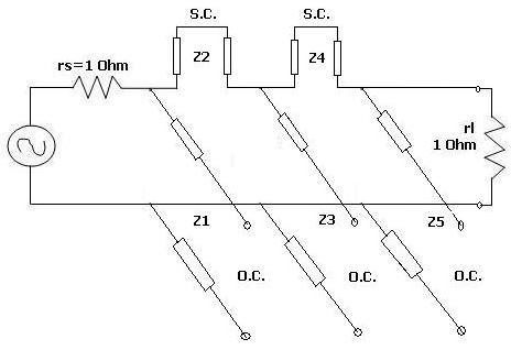
In the figure above, a unit element is inserted at the input and output without changing the rest of the elements. Now Z1 and Z5 are converted from open circuit shunt elements to short circuit series elements.
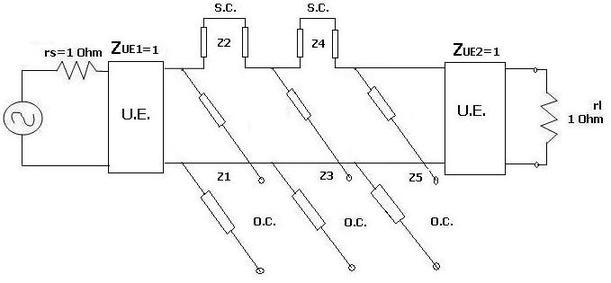
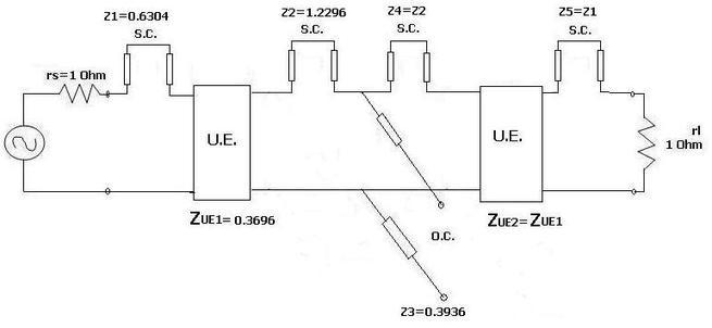
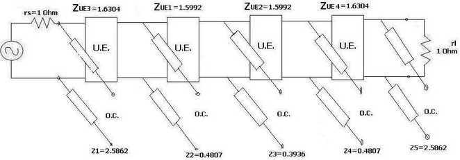
Now two more unit elements are inserted at the source and destination. Using Kuroda’s identities, z1, z2, z4, and z5 elements are converted from S.C. series elements to O.C. shunt elements.
The same RF filter design is incorporated using built-in microstrip line elements in RF/microwave design software such as Agilent EESoF or ADS or Microwave Office from AWR.
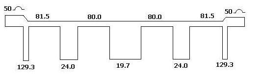
Step 4: Following is the realization of the RF filter as microstrip based on specifications mentioned at the beginning of this article.
Step 5: This microstrip layout is etched on the respective dielectric based on the frequency of operation as mentioned and tested with connectors using a scalar network analyzer (SNA).
Conclusion
The same design approach or method can be applied to RF bandpass filter design and other types. It’s important to select the filter order “N” as per the normalized frequency versus attenuation curve. Based on this filter order “N”, appropriate filter coefficients must be extracted from the table as per the desired ripple.
Advertisement


