RF
RFSpectral Analysis in Python with DSP Libraries
Advertisement
This page explains how to perform spectral analysis in Python, utilizing Python DSP libraries to analyze time-domain signals.
Introduction
Signal parameters can be measured in either the time domain or the frequency domain. Signals come in various shapes and sizes, like sine waves, square waves, rectangular waves, random binary sequences, pulses, and random noise. They can be periodic or aperiodic based on their repetition over time.
Spectral analysis involves measuring, plotting, and analyzing a signal’s spectrum in both the time and frequency domains. Time-domain analysis is often done with an oscilloscope, where the X-axis represents time and the Y-axis represents amplitude. Frequency-domain analysis can be done with a spectrum analyzer, where the X-axis represents frequency and the Y-axis represents power or amplitude.
Both time and frequency domain analysis can be performed in software like MATLAB, Labview, or Python. The Inverse Fast Fourier Transform (IFFT) converts a frequency-domain signal vector into a time-domain vector. The Fast Fourier Transform (FFT) or Discrete Fourier Transform (DFT) converts a time-domain signal vector into a frequency-domain signal vector. Therefore, spectral analysis in Python is straightforward, thanks to the built-in functions in various toolkits.
Spectral Analysis Python Script
The following Python code provides time and frequency domain plots useful for spectral analysis of signals:
from scipy.fftpack import fft, ifft
import numpy as np
import matplotlib.pyplot as plt
from scipy import signal
fc = 1000 # frequency of the carrier
N = 1e3
fs = 10 * fc # sampling frequency with oversampling factor=10
time = np.arange(N) / fs
x = np.sin(2 * np.pi * fc * time) # time domain signal (real number)
plt.figure()
plt.plot(time, x)
plt.xlabel('Time')
plt.ylabel('Signal amplitude')
plt.title('Time domain signal amplitude versus time samples')
N1 = 256 # FFT size
X1 = fft(x, N1) # N-point complex DFT, output contains DC at index 0
# calculate frequency bins with FFT
# Power spectral density (PSD) using FFT and absolute squared
df = fs / N1 # frequency resolution
sampleIndex = np.arange(start=0, stop=N1) # raw index for FFT plot
f = sampleIndex * df # x-axis index converted to frequencies
PSD = abs(X1)**2
n1 = len(f) // 2
n2 = len(PSD) // 2
plt.figure()
plt.plot(f[1:n1], PSD[1:n2])
plt.xlabel('Frequency indices')
plt.ylabel('Signal power')
plt.title('Frequency domain signal power vs frequency indices')
# Power spectral density (PSD) using signal.welch
f1, Pxx_spec = signal.welch(x, fs, 'flattop', 512, scaling='spectrum')
plt.figure()
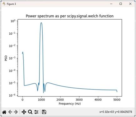
plt.semilogy(f1, np.sqrt(Pxx_spec))
plt.xlabel('Frequency (Hz)')
plt.ylabel('PSD')
plt.title('Power spectrum as per scipy.signal.welch function')
plt.show()
Spectrum Analysis in Python Output Plots
The code above generates the following plots:
- Time-domain waveform (Amplitude vs. time)
- Instantaneous power vs. time waveform (Power vs. time)
- Frequency-domain waveform (Power vs. frequency)
- Using FFT
- Using
signal.welchfunction
Amplitude vs Time Plot

Power vs Frequency Plot using FFT

Power vs Frequency Plot using Welch
Other plots provide more insights when the signal contains complex baseband information with advanced modulation schemes such as OFDM, OFDMA, 16QAM, 64QAM, 256QAM, 1024QAM, etc. These plots include: EVM (Error Vector Magnitude) vs. symbols, EVM vs. subcarriers, Constellation IQ diagram, CCDF, channel frequency response, spectral flatness, jitter (measured in the time domain), and phase noise (measured in the frequency domain).